cs61b-Data Structure

Data Structures

Some Resources

• Big-O Cheat Sheet

Tree

1. A tree consists of:
   • A set of nodes.
   • A set of edges that connect those nodes.
     • Constraint: There is exactly one path between any two nodes

2. Rooted Tree and Rooted Binary Trees
   In a rooted tree, we call one node the root.
   • Every node N except the root has exactly one parent, defined as the first node on the path from N to the root.
   • A node with no child is called a leaf
     In a rooted binary tree, every node has either 1, 0, or 2 children
     

Tree Traversal

Traversal Orderings

1. Level Order

• Visit top-to-bottom, left-to-right

2. Depth First Traversals

• 3 types: Preorder, Inorder, Postorder

Depth First Traversals

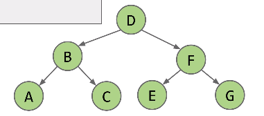
1. preOrder (root-left-right)
   The result of preOrder for the above tree is D B A C F E G

preOrder(BSTNode x) {
  if (x == null) return;
  print(x.key)
  preOrder(x.left)
  preOrder(x.right)
}

2. Inorder (left-root-right)
   the result of preOrder for the above tree is A B C D E F G

inOrder(BSTNode x) {
  if (x == null) return;
  preOrder(x.left)
  print(x.key)
  preOrder(x.right)
}

3. Postorder (left-right-root)
   the result of preOrder for the above tree is A C B E G F D

inOrder(BSTNode x) {
  if (x == null) return;
  preOrder(x.left)
  preOrder(x.right)
  print(x.key)
}

Binary Search Tree (BST)

BST Definition

A binary search tree is a rooted binary tree with the BST property

BST Property. For every node X in the tree:

• Every key in the left subtree is less than X’ key
• Every key in the right subtree is greater than X’s key

Three rules: Complete, Transitive and Antisymmetric.
One consequence of these rules: No duplicate keys allowed!

BST Operations

1. Search
   • Start at the root and compare it with the search element.
   • if X > element, move on the root’s right child.
   • if X < element, move on the root’s left child.
   • repeat process recursively until find the item or get to a leaf in which case the tree does not contain the item

static BST find(BST T, Key sk) {
   if (T == null)
      return null;
   if (sk.equals(T.key))
      return T;
   else if (sk ≺ T.key)
      return find(T.left, sk);
   else
      return find(T.right, sk);
}

2. Insert

• First, search in the tree for node. If find it, do nothing.
• if don’t find it, we will be at the leaf node, add the new element

static BST insert(BST T, Key ik) {
  if (T == null)
    return new BST(ik);
  if (ik ≺ T.key)
    T.left = insert(T.left, ik);
  else if (ik ≻ T.key)
    T.right = insert(T.right, ik);
  return T;
}

3. Delete
   Three cases:
   1. no children
      It is a leaf, just delete its parent pointer.
      Example: delete(“flat”):
      
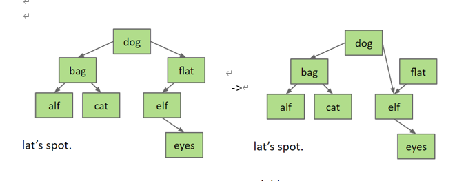
   2. one children
      Reassign the parent’s child pointer to the node’s child.
      Example: delete(“flat”):
      
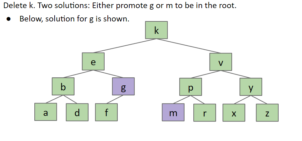
   3. two children
      Two solutions: Use it’s right child’s rightest node or it’s left child’s leftest node to replace it.
      For example: delete k. use ‘g’ or ‘m’ to replace k.
      

Height and Depth

Height and average depth are important properties of BSTs

• The depth of a node is how far it is from the root. e.g. depth(g) = 2
• The height of a tree is the depth of its deepest leaf, e.g. height(T) = 4
• The average depth of a tree is the average depth of a tree’s nodes e.g. (0x1 + 1x2 + 2x4 + 3x6 + 4x1) / (1+2+4=6+1) = 2.35

Height abd average depth determine runtimes for BST operations

• The height of a tree determines the worst case runtime to find a node.
  • Example: Worst case is contains(s), requires 5 comparisons (height+1)
• The average depth determines the average case runtime to find a node.
  • Example: Average case is 3.35 comparisons (average depth + 1).

B-trees / 2-3 trees / 2-3-4 trees

Insertion

To get a balanced (bushy) tree, which will prevent the worst case runtime of N in BSTs, we never add a leaf node. Just add to a current leaf node. Like following figure:

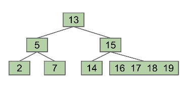
But this idea will degenerate a linked list at last which will lead to a runtime of $N$ again.

Solution: Set a limit on the number of elements in a single node. Like L = 3. If we add a new element to a node when it already has 3 elements, we will split the node in half by bumping up the middle left node. Like following figure:

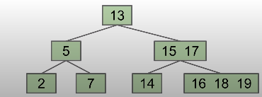
These trees called 2-3-4 or 2-3 trees

• B-trees of order L = 3 called a 2-3-4 tree or a 2-4 tree
  • “2-3-4” refers to the number of children that a node can have. e.g. a 2-3-4 tree node may have 2, 3, or 4 children.
• B-trees of order L = 2 called a 2-3 tree
  

And here is a B-tree Visualization tool can generate the processing of creation of different b trees:https://www.cs.usfca.edu/~galles/visualization/BTree.html

Because of the way B-Trees are constructed, we get two nice invariants:

• All leaves must be the same distance from the source.
• A non-leaf node with k items must have exactly k+1 children

Deletion

Deletion Operations

LLRB (Left Leaning Red Black Tree)

There are many types of search trees:

• Binary search trees : Can balance using rotation
• 2-3 trees: Balanced by construction (no rotations required)

How about build a BST that is stucturally identical to 2-3 tree?

A 2-3 tree with only 2-nodes is the same as BST. How about three nodes?

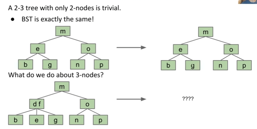
We create a “glue” link with the smaller item off to the left, and mark it as "red"

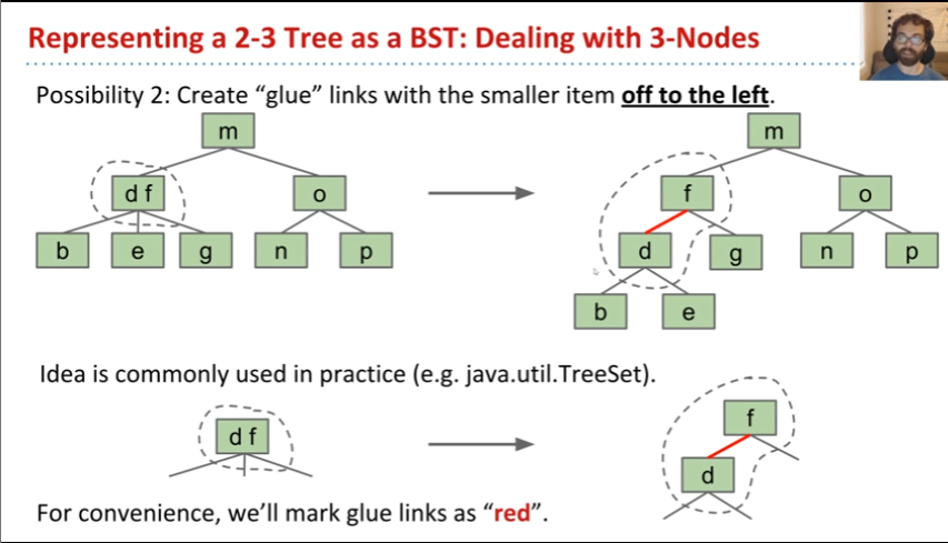
A BST with left glue links that represents a 2-3 trees is often called a “Left Leaning Red Black Binary Search Tree” or LLRB

• LLRBs are normal BSTs!
• There is a 1-1 correspondence between LLRB and an equivalent 2-3 tree.
• The red is just a convenient fiction. Red links don’t “do” anything special.

LLRB Height

Suppose we have a 2-3 tree of height H.

• What is the maximum height of the corresponding LLRB?
  • Total height is H(black) + H(red) + 1(red) = 2H +1

LLRB property

• No node has two red links
• Every path from root to a leaf has same number of black links.

LLRB Construction

• Insert as usual into a BST
• Use zero or more rotations to maintain the 1-1 mapping

LLRB Insertion

• We always insert red link
• If there is a right leaning “3-node”, we have a Left Leaning Violation
  • Rotate left the appropriate node to fix
• If there are two consecutive left links, we have an Incorrect 4 Node Violation.
  • Rotate right the appropriate node to fix
• If there are any nodes with two red children, we have a Temporary 4 Node.
  • Color filp the node to emulate the split operation.

Rules and Demo

• Rigth red link -> rotate left.
• Two consecutive left links -> rotate right.
• Red left and red right -> color flip.

Demo: Insert 1-7 to empty LLRB

Hash Table

Start with “DataIndexedIntegerSet”

Suppose we create an ArrayList of type boolean and size 2 billion. Let everything be false by default.

• The add(int x) method simply sets the x position in ArrayList to true.
• The contains(int x) method simply returns whether the x position in ArrayList is true or false

public class DataIndexedIntegerSet {
    private boolean[] present;

    public DataIndexedIntegerSet() {
        present = new boolean[2000000000];
    }

    public void add(int x) {
        present[i] = true;
    }

    public boolean contains(int x) {
        return present[i];
    }

Problem of above approach:

• Extremely wasteful. If 1 byte per boolean, the above needs 2GB. And user may only insert handful items.
• What do we do if we want to insert a String?

Solving the word-insertion problem

Now we want to insert the String to the ArrayList, How that works?

Use Integer to represent String

We can use the idea of how number system works:
A four digit number, say 5149, can be written as

$5 * 10^3 + 1 * 10^2 + 4 * 10^1 + 9 * 10^0$

Similarly, there are 26 letters in the english lowercase alphabet. We use 26 as the multiplier. And give each letter a number like : $a = 1, b = 2, c = 3, ...., z = 26$ Then the "cat" can be represented as:

$3 * 26^2 + 1 * 26^1 + 20 * 26^0$

Code will be like:

public class DataIndexedEnglishWordSet {
    private boolean[] present;

    public DataIndexedEnglishWordSet() {
        present = new boolean[2000000000];
    }

    public void add(String s) {
        present[englishToInt(s)] = true;
    }

    public boolean contains(int i) {
        resent present[englishToInt(s)];
    }
}

public static int letterNum(String s, int i) {
    /** Converts ith character of String to a letter number.
    * e.g. 'a' -> 1, 'b' -> 2, 'z' -> 26 */
    int ithChar = s.charAt(i)
    if ((ithChar < 'a') || (ithChar > 'z')) {
        throw new IllegalArgumentException();
    }

    return ithChar - 'a' + 1;
}

public static int englishToInt(String s) {
    int intRep = 0;
    for (int i = 0l i < s.length(); i += 1) {
        intRep = intRep * 26;
        intRep += letterNum(s, i);
    }

    return intRep;
}

Integer Overflow and Hash code

In Java, the largest possible integer is 2,147,483,647. If you go over this limit, you overflow, starting back over at the smallest integer, which is -2,147,483,648. In other words, the next number after 2,147,483,647 is -2,147,483,648.

Due to above limitation, we will get wrong number, For example:

• With base 126, we will run into overflow even for short strings.
  • “omens” = 28,196,917,171, which is much greater than the maximum integer!
  • asciiToint('omens') will give us -1,867,853,901 instead. And it can result in collisions like following picture
    

The official explanation of hash code: a hash code “projects a value from a set with many (or even an infinite number of) members to a value from a set with a fixed number of (fewer) members.”

Pigeonhole Principle tell us that if there are more than X possible items (X > container capacity), multiple items will share the same hash code.

10 pigeons, 9 boxes, two in one hole.

Hash Table

Suppose N items have the same numerical representation h, we store a “bucket” of these N item at position h. The implementation of this bucket could use ArrayLists, LinkedList, ArraySet, and ect.

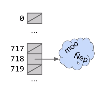
Each bucket in array is initially empty, When an item x gets added at the index h:

• if bucket h is empty, we create a new list containing x and store it at index h
• if bucket h i already a list, we add x to this list if it is not already present.
  

To improve it, we can use modulus of hahscode to reduce bucket count.

The data structure we’ve just created here is called a hash table.

• Data is converted by a hash function into an integer representation called a hash code
• The hash code is then reduced to a valid index, usually using the modulus operator.
  

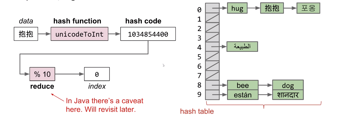
Q: What’s the runtime of current hash table?
A: $\theta(Q)$, where Q is the length of the longest list.

Improve performance of Hash Table

There are two ways to improve the performance:

• Dynamically growing our HashTable
• Improving our HashCodes

Dynamically growing the hash table

Suppose we have $M$ buckets and $N$ items. Then our load factor is $N/M$. N Keeps increasing, so we need to increasing M to make our load factor lower.

For Example:
When $N/M$ is >= 1.5, then double M.

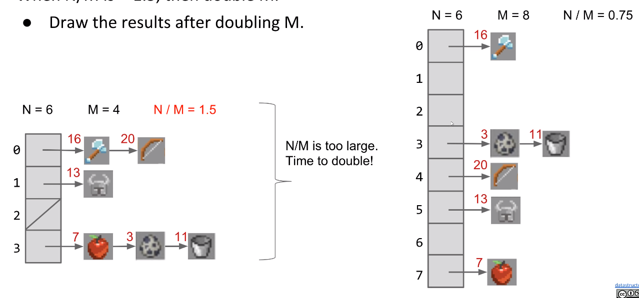
As long as M = $\theta(N)$, then $O(N/M)$ = $O(1)$, Assuming items are evenly distributed, lists will be approximately $N/M$ long, resulting in $\theta(N/M)$ runtimes.

But, one important thing to consider is the cost of the resize operation.

• Resizing takes $\theta(N)$ time. Have to redistribute all items.
• Most add operations will be $\theta(1)$. Some will be $\theta(N)$ time for resizing.

However, there still some flaws for resizing.
Both tables below have load factor of 1. But left table is much worse.

Good HashCode function

A typical hash code base is a small prime.

• Prime can avoid the overflow issue
• Lower chance of resulting hashCode having a bad relationship with the number of buckets
• Small prime is lower cost to compute.

Heap

Heap is a special data structure which is usually used to solve the priority queue problem.

• Priority queue: It is a ADT that optimizes for handling The maximum or minimum elements. Think about this scenario : We want to return the 10 tallest students in a big class. After we adding 10 students, when we add the 11th student, we remove the smallest one out to keep 10 students until we check all the students’ height.

Heap includes min-heap and max-heap. A heap has two properties:

• Min/Max heap: Every node is less/bigger or equal to both of its children
• Complete: Missing items only at the bottom level (if any), all nodes are as far left as possible

For Example:

The green two three are heaps, and the red twos aren’t.

Heap Operations

Animated demo of below operations

Add

When we insert X into the following heap, the processing will be :

• Add to end of heap temporarily.
• Swim up the hierarchy to its right place.

getSmallest

The root is the smallest one. So return the item in the root node.

removeSmallest

• Swap the last item in the heap into the root.
• Sink down the hierarchy to the proper place.

Heap Implementation

Due to heap hast the “complete” property. So we can number the tree from top to bottom and left to right. Then use an array to store the key which the index indicates the position of every node.

For convenient, offsetting everything by 1 spot.

It makes computation of children/parent simply:

• leftChild(k) = k*2
• rightChild(k) = k*2+1
• parent(k) = k/2

Graph

A graph consists of:

• A set of vertices (a.k.a nodes).
• A set of zero or more edges, each of which connects two nodes.
  

Simple Graph

A simple graph is a graph with:

• No edges that connect a vertex to itself, i.e. no “loops”
• No two edges that connect the same vertices, i.e. no “parallel edges”
  

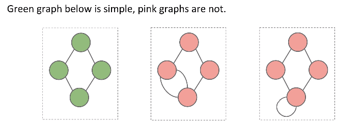
More types and Terminology:

• Directed graph
• Undirected graph
• acyclic graph
• cyclic graph
• With Edge Labels graph

There are directed graphs, where the edge (u, v) means that the edge starts at u, and goes to v (and the vice versa is not true, unless the edge (v, u) also exists.) Edges in directed graphs have an arrow.

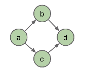
There are undirected graphs, where an edge (u, v) can mean that the edge goes from the nodes u to v and from the nodes v to u too.

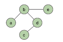
There are also acyclic graphs. These are graphs that don’t have any cycles.

And then there are cyclic graphs, i.e., there exists a way to start at a node, follow some unique edges, and return back to the same node you started from.

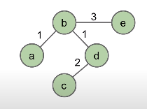
• Graph:
  • Set of vertices, a.k.a nodes.
  • Set of edges: Paris of vertices.
  • Vertices with an edge between are adjacent
  • Vertices or edges may have labels (or weights)
• A path is a sequence of vertices connected by edges
• A cycle is a path whose first and last vertices are the same.
• Two vertices are connected if there is a path between them. If all vertices are connected, we say the graph is connected.

Graph Representations

1. Adjacency Matrix

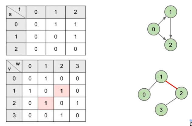
• G.adj(2) would return an iterator where we can call next() up to two times
  • next() returns 1
  • next() returns 3
• Total runtime to iterate over all neighbors of v is $\Theta(V)$
  • underlying code has to iterate through entire array to handle next() and hasNext() calls.

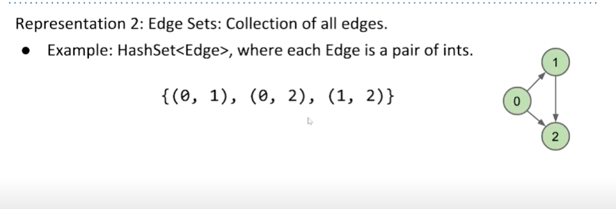
2. Edge Sets: Collection of all edges
   

3. Adjacency lists

• Common approach: Maintain array of lists indexed by vertex number.
• Most popular approach for representing graphs.
  

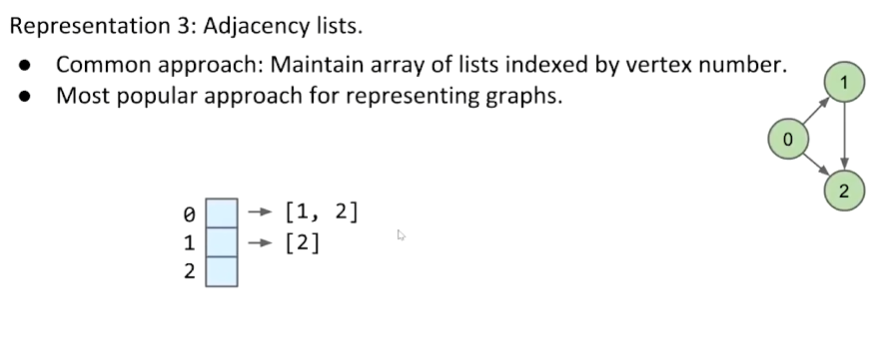
Runtime of some operations for each representation:

DFS & BFS

s-t Connectivity

write a function connected(s,t) that takes in two vertices and returns whether there exists a path between the two.

The process is that:

1. Mark the current vertex.
2. Does s==t? if so, return true.
3. Otherwise, if connected(v,t) for any unmarked neighbor v of s, return true.
4. Return false.

These slides shows the detail of above process

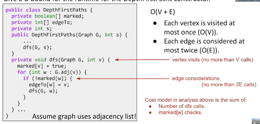
Depth First Traversal

Goal: Find a path from s to every other reachable vertex, visiting each vertex at most once. dfs(v) is as follows:

• Mark v.
• For each unmarked adjacent vertex w:
  • set edgeTo[w] = v.
  • dfs(w)

DFS Demo

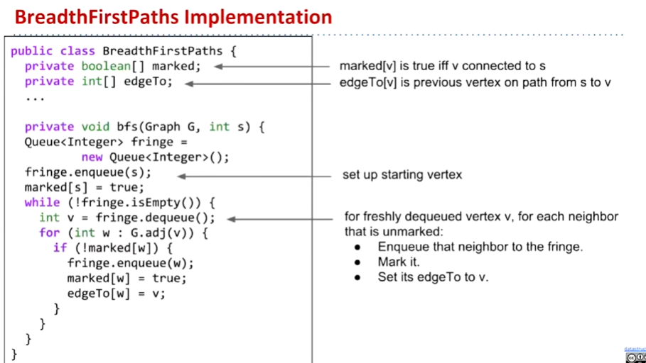
Breadth First Traversal

DFS DEMO

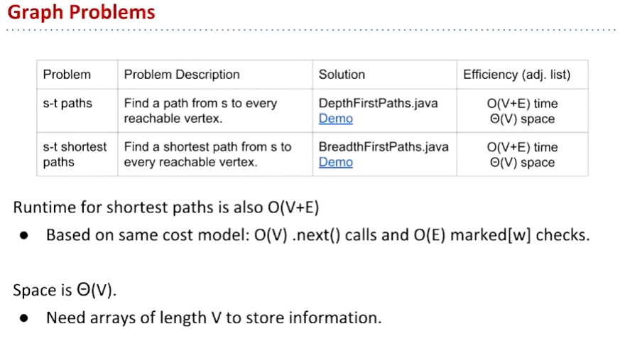
Summary of DFS and BFS

Dijkstra’s Algorithm

• Insert all vertices into fringe PQ (Priority Queue), storing vertices in order of distance from source.
• Repeat: Remove (closest) vertex v from PQ, and relax all edges pointing from v.

Dijkstra’s Algorithm Demo Link

Pseudocode

def dijkstras(source):
  PQ.add(source, 0)
  For all other vertices, v, PQ.add(v, infinity)
  while PQ is not empty:
    p = PQ.removeSmallest()
    relax(all edges from p)

def relax(edge p,q):
  if q is visited (i.e., q is not in PQ):
    return
  if distTo[p] + weight(edge) < distTo[q]:
    distTo[q] = distTo[p] + w
    edgeTo[q] = p
    PQ.changePriority(q, distTo[q])

• Key invariants:
  • edgeTo[v] is the best known predecessor of v.
  • distTo[v] is the best known total distance from source to v.
  • PQ contains all unvisited vertices in order of distTo.
• Important properties:
  • Always visits vertices in order of total distance from source.
  • Relaxation always fails on edges to visited (white) vertices.

A star algorithm

Demo

Minimum Spanning Trees

Spanning Trees

Given an undirected graph, s spanning tree T is a subgraph of G, where T:

• Is connected
• Is acyclic
• Includes all of the vertices

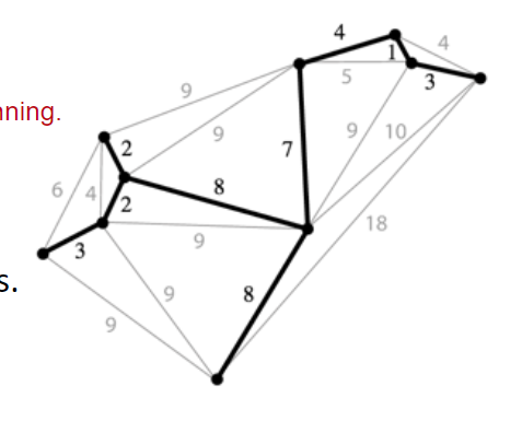
A minimum spanning tree is a spanning tree of minimum total weight

sometimes, the MST happens to be an SPT for a specific vertex.

Cut Property

• A Cut is an assignment of a graph’s nodes to two non-empty sets.
• A crossing edge is an edge which connects a node from one set to a node from the other set.

Cut property: Given any cut, minimum weight crossing edge is in the MST.

Proof:
Suppose that the minimum crossing edge $e$ were not in the MST. Since it is not a part of the MST, if we add that edge, a cycle wil be created. Then there must exists a crossing edge $f$ which crosses back over. Thus, we can remove $f$ and keep $e$, and this will give us a lower weight spanning tree which is a contradiction.

Prim’s Algorithm

Start from some arbitrary start node.

• Repeatedly add shortest edge(mark black) that has one node inside the MST under construction.
• Repeat until V-1 edges.

Prim’s Algorithm Demo

Prim’s Algorithm implementation (more efficient)

Use Priority Queue
Demo

runtime: O(V * log(V) + V * log(V) + E * log(V))

Kruskal’s Algorithm

Consider edges in order of increasing weight. Add to MST unless a cycle is created.

• Repeat until V-1 edges.

Kruskal’s Demo

Kruskal’s Algorithm implementation

Use Priority Queue.
Demo

runtime: O(E logE)

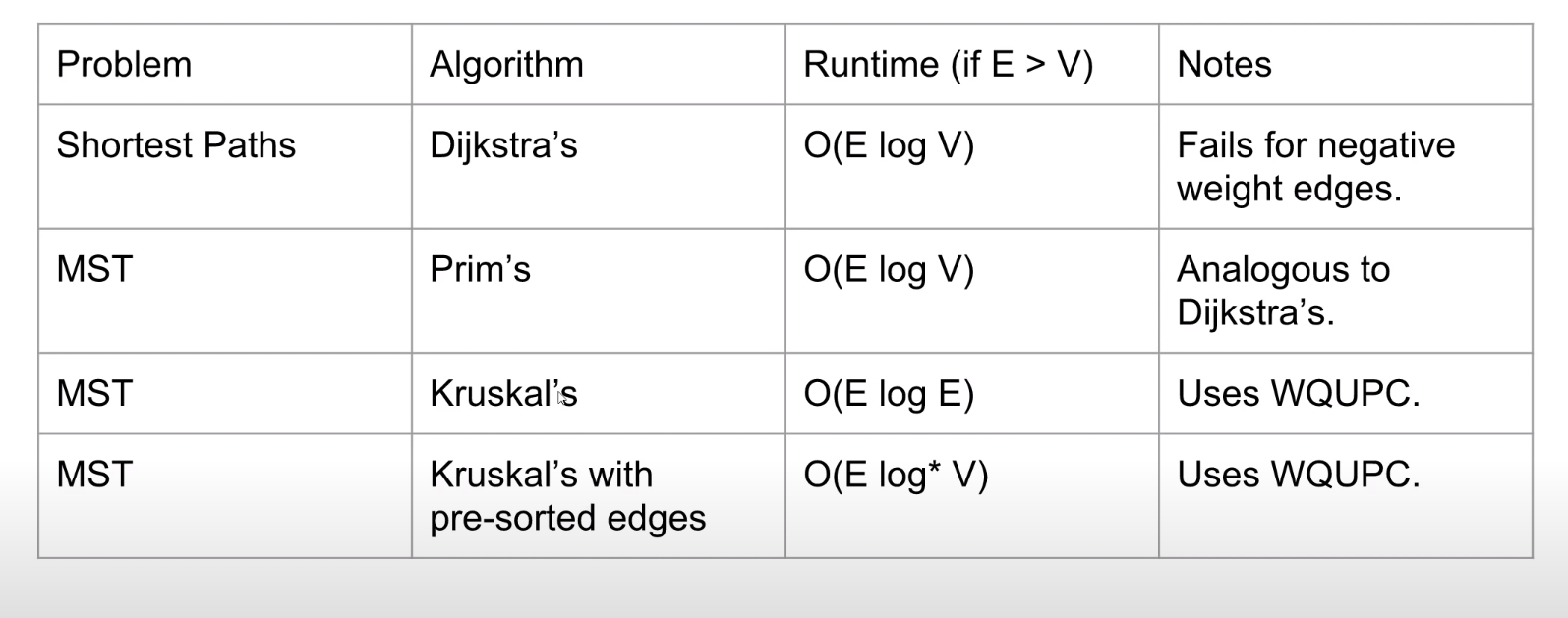
Shortest Paths and MST Algorithms Comparison

Range Searching

QuadTrees

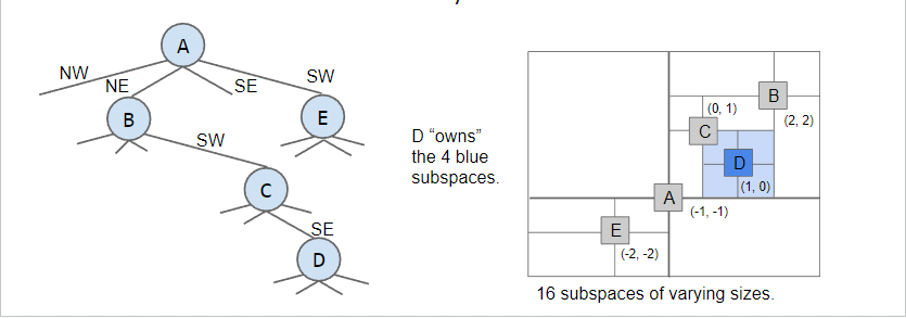
Quadtrees are a form of “spatial partitioning”

• Quadtrees: Each nodes “owns” 4 subspaces
  • Space is more finely divided in regions where there are more points
  • Results in better runtime in many circumstances

QuadTrees Demo

Ranges Search using a QuadTree

Demo

K-D Trees

2D Trees Demo

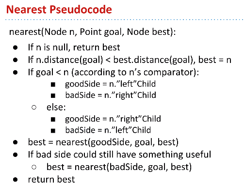
Nearest Neighbor using a K-D Tree

Demo

Pseudocode:

Trie

Tries are a very useful data structure used in cases where keys can be broken into “characters” and share prefixes with other keys (e.g. strings)

Suppose we have “sam”, “sad”, “sap”, “same”, “a”, and “awls” and construct a trie:

• Every node stores only one letter
• Nodes can be shared by multiple keys

It will be like：

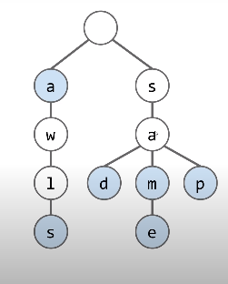
The blue nodes means the end of the key.

For example:
contains(“sa”) will be false cause “a” node is white which is not the end of a key.
contains(“a”) will be true, blue node.

Insertion animated demo

The implementation of tries

The basic implementation of tries

1. DataIndexedCharMap

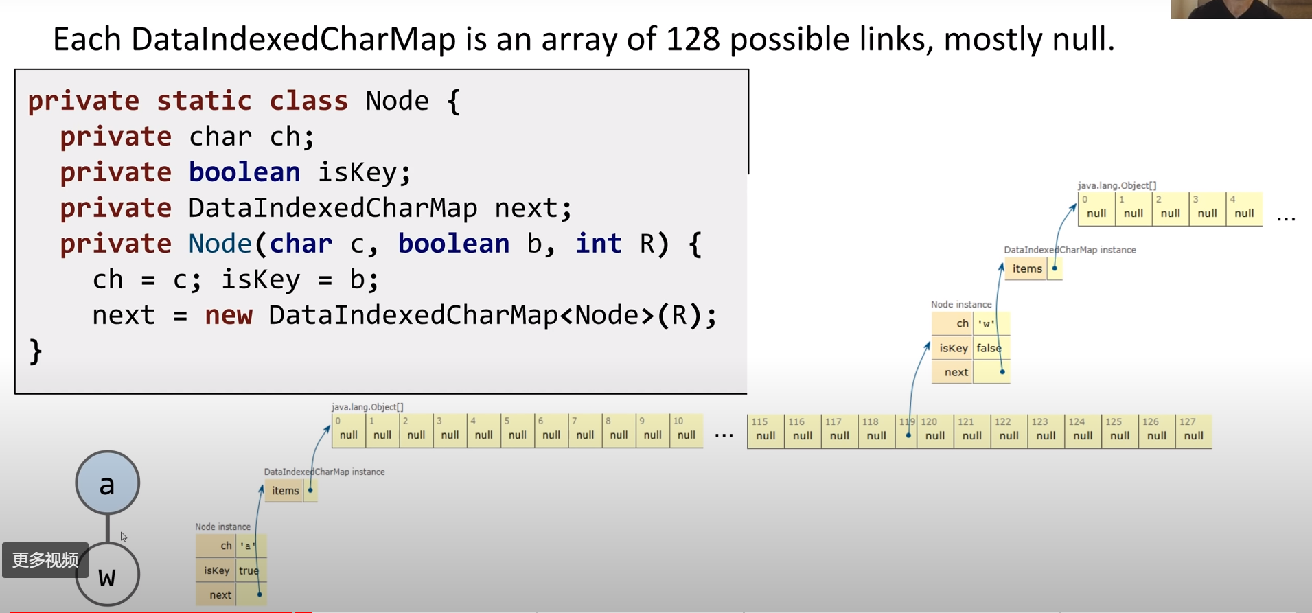
public class TrieSet {
   private static final int R = 128; // ASCII
   private Node root;    // root of trie

   private static class Node {
      private char ch;  //this line could be removed
      private boolean isKey;   
      private DataIndexedCharMap next;

      private Node(char c, boolean blue, int R) {
         ch = c; //this line could be removed
         isKey = blue;
         next = new DataIndexedCharMap<Node>(R);
      }
   }
}

2. Hash-Table based Trie

Hash-Table based Trie. This won’t create an array of 128 spots, but instead initialize the default value and resize the array only when necessary with the load factor.

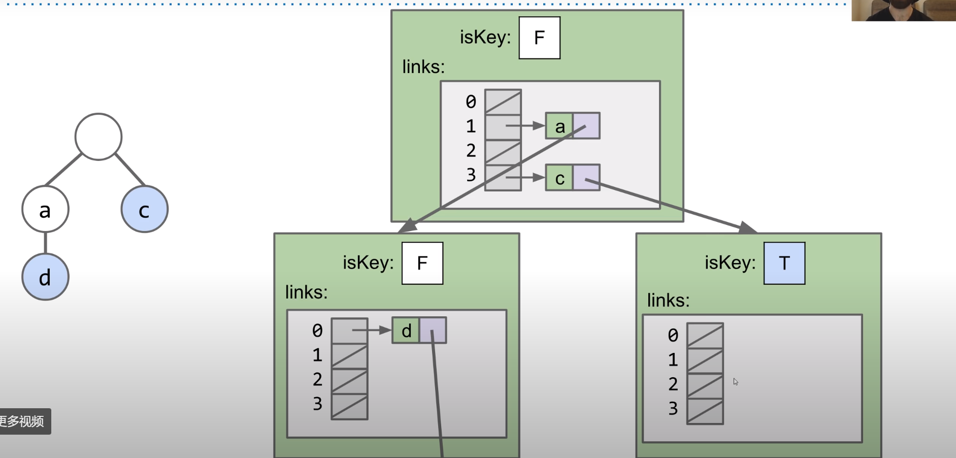
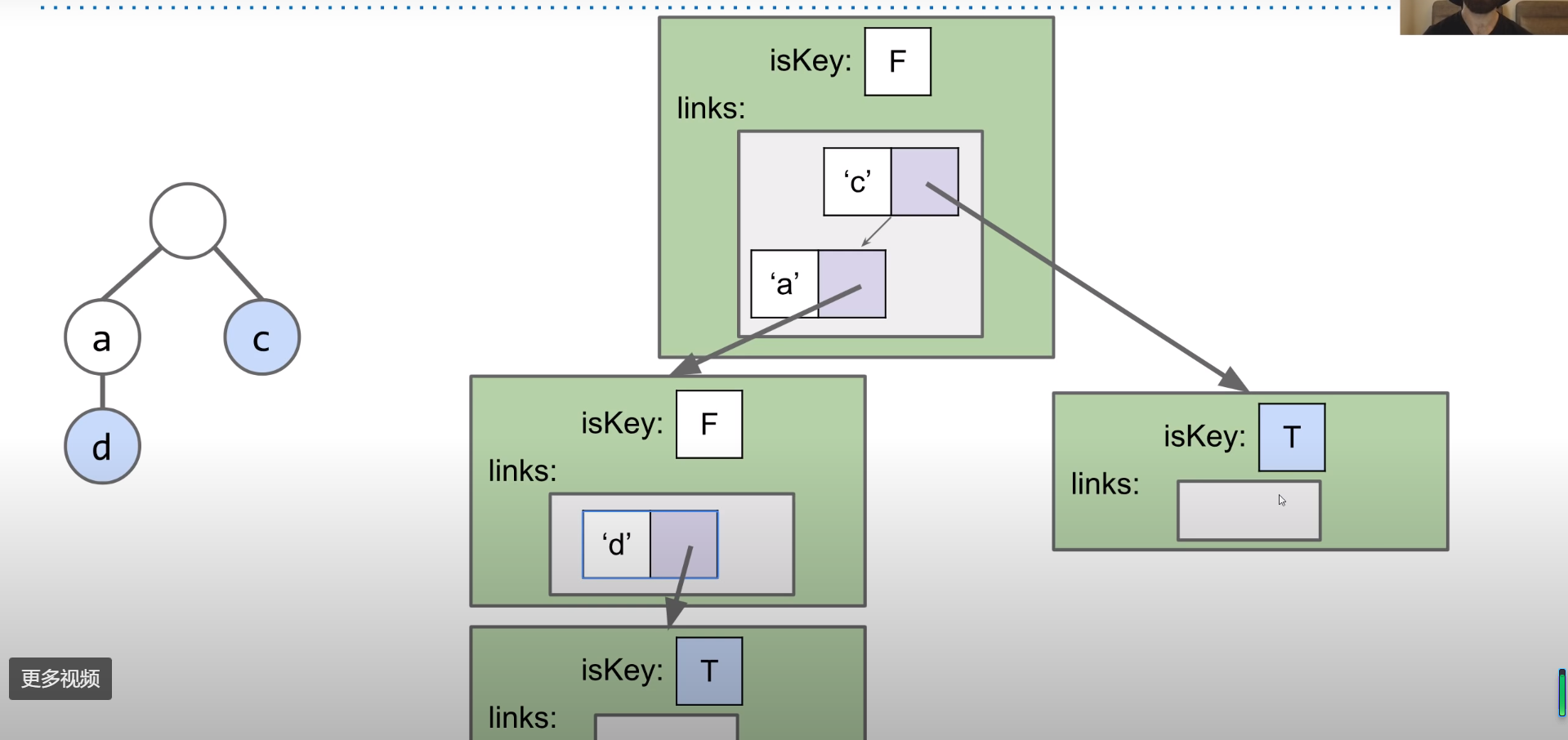
3. BST based Trie

BST based Trie. Again this will only create children pointers when necessary, and we will store the children in the BST. Obviously, we still have the worry of the runtime for searching in this BST, but this is not a bad approach.

String Operations

Prefix Matching

Tries can support many string operations efficiently.
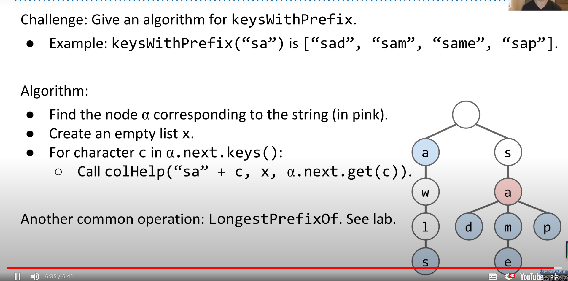
Like keyWithPrefix, we can traverse to the end of the prefix and return all remaining keys in the trie.

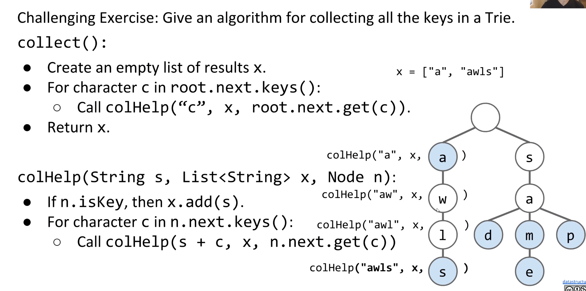
Let’s attempt to define a method collect which returns all of the keys in a Trie. The pseudocode will be as follows:

collect():
    Create an empty list of results x
    For character c in root.next.keys():
        Call colHelp(c, x, root.next.get(c))
    Return x

colHelp(String s, List<String> x, Node n):
    if n.isKey:
        x.add(s)
    For character c in n.next.keys():
        Call colHelp(s + c, x, n.next.get(c))

KeyWithPrefix function will be :

keysWithPrefix(String s):
    Find the end of the prefix, alpha
    Create an empty list x
    For character in alpha.next.keys():
        Call colHelp("sa" + c, x, alpha.next.get(c))
    Return x

Autocomplete

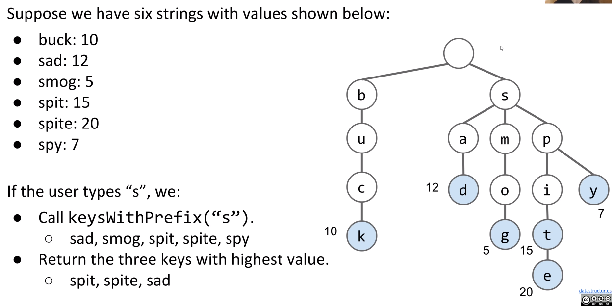
When you type into any search browser, for example Google, there are always suggestions of what you are about to type.

One way to achieve this is using a Trie. We will build a map from strings to values.

• Values will represent how important Google thinks that string is
• Store billions of string efficiently since they share nodes.
• When a user types a query, we can call the method keysWithPrefix(x) and return the top 10 strings

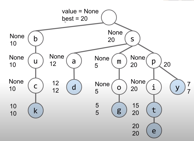
One major flaw with this system is if the user types in short length strings. The results will be huge amount. A possible solution to this issue is to store the best value of a substring in each node.

Topological Sort

Suppose we have a collection of different tasks or activities, some of which must happen before another. How do we find sort the tasks such that for each task $v$, the tasks that happen before $v$ come earlier in our sort?

We can first view our collection of tasks as a graph in which each node represents a task.
An edge $v->w$ indicates that $v$ must happen before $w$. Now our original problem is reduced to finding a topological sort.

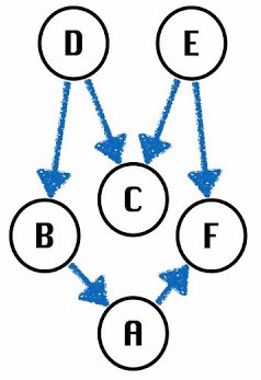
The Valid orderings include: [D,B,A,E,C,F], [E,D,C,B,A,F]

Note that topological sorts only apply to directed, acyclic (no cycles) graphs - or DAGs

Topological Sort: an ordering of a DAG’s vertices such that for every directed edge $u->v$, $u$ comes before $v$ in the ordering.

For any topological ordering, you can redraw the graph so that the vertices are all in one line.

Topological Sort Algorithm

Topological Sort Algorithm:

• Perform a DFS traversal from every vertex in the graph, not clearing markings in between traversals.
• Record DFS postorder along the way.
• Topological ordering is the reverse of the postorder.

Demo

Pseudocode:

topological(DAG):
    initialize marked array
    initialize postOrder list
    for all vertices in DAG:
        if vertex is not marked:
            dfs(vertex, marked, postOrder)
    return postOrder reversed

dfs(vertex, marked, postOrder):
    marked[vertex] = true
    for neighbor of vertex:
        dfs(neighbor, marked, postOrder)
    postOrder.add(vertex)

Runtime: $O(V+E)$ where V and E are the number of nodes and edges in the graph.

Shortest Paths on DAGs

Use topological order we can deal with negative value.

• Visit vertices in topological order
• On each visit, relax all outgoing edges.

Demo

runtime: $O(V+E)$

Longest Paths Problem

Finding the longest path tree (LPT) from s to every other vertex. The path must be simple (no cycles!)

With DAGs, we can do:

• Form a new copy of the graph, called G’, with all edge weights negated (signs flipped).
• Run DAG shortest paths on G’ yielding result X
• Flip the signs of all values in X.distTo. X.edgeTo is already correct.