Terrain Analysis

Digital Terrain Model

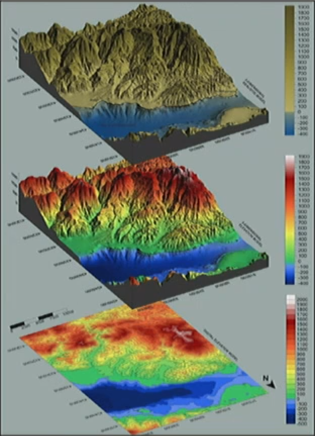
Digital Elevation Model(DEM)

A grid of bare-earth elevation values referenced to a horizontal and vertical datum
Continuous surface (Raster) of topography
Different scales; global coverage at 30m; regional coverage at 10m and some at 3m; US 1m resolution

DEM from Raster to TIN Vector

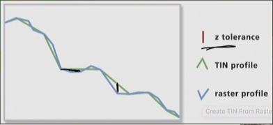
Tin model – continuous vector (triangles)
Z tolerance: a acceptable gap between two profiles

Digital Terrain Model (DTM)

In the US, it means a vector dataset that can be used to create a DEM via interpolation and can augment a DEM

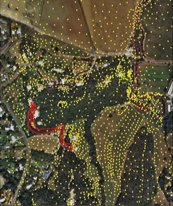
DTM Mass Points and Breaklines

Breaklines (red lines in the figure) record discontinuities or sudden changes in the surface
Mass points are point elevation values

Digital Surface Model (DSM)

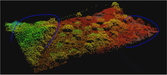
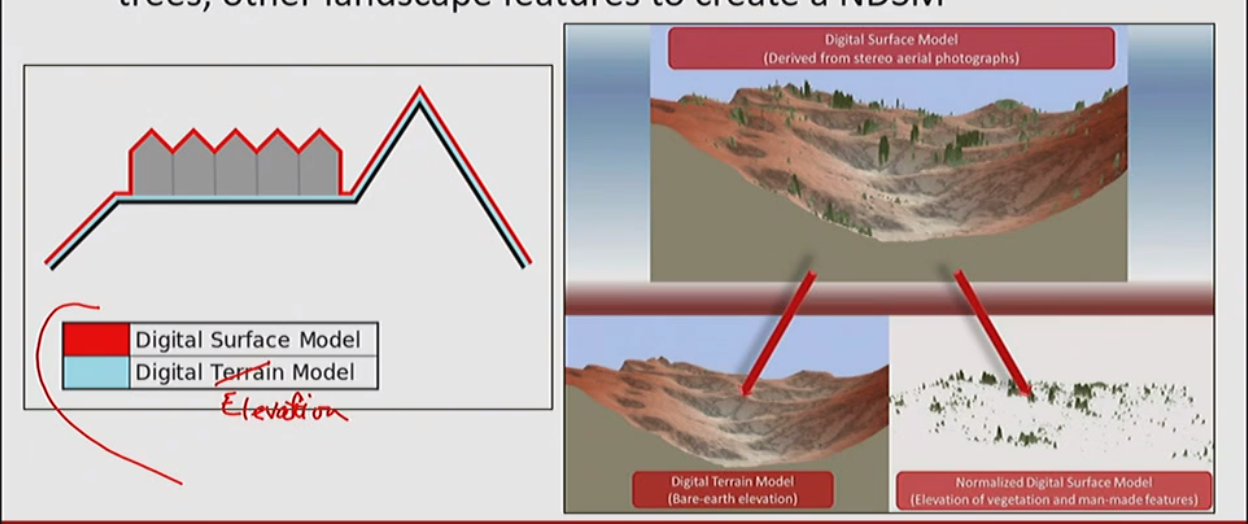
True 3D surface including buildings, trees, and other landscape features

Normalized Digital Surface Model (NDSM)

Difference between DEM and DSM for height for buildings, trees, other landscape features to create a NDSM

Land Surface Parameters

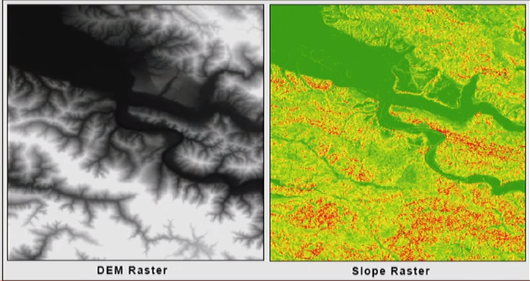
Slope

The rate of change in elevation for each cell in a DEM; measured in degrees, up to 90 degree, or percent; rise/run

Aspect (方位)

What compass direction a slope is facing; raster values are degrees of compass direction(0-360) or 1 for flat earth

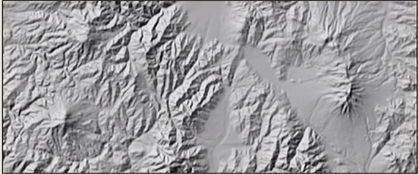
Hillshade (山体阴影)

A grayscale 3D representation of the elevation of the surface; taking into account the sun’s relative position for shading the image.
Inputs: DEM; Azimuth and altitude (to specify the sun’s position); optionally, z-factor for scaling to add vertical exaggeration for visual effect

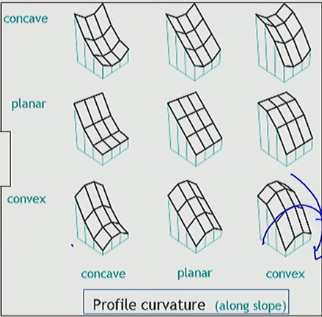
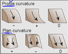
Profile Curvature and Plan Curvature

Curvature of landscape feature along the slope plane(profile) and across the scope plane(plan)

Viewshed

Creates the area where an observer can see objects on the ground (or from the ground to a certain point); resultant raster is the number of times that each cell location in the input surface can be seen by the input observation point

Hydrologic Analysis: Flow Direction

Flow direction: assessment of direction water will move over the surface. Algorithms are designed which check steepness of a cell and its neighbors. This is complicated; topic of on-going research
Flow accumulation: calculates water accumulation based on a flow direction raster
Fill sinks: in reality, small depressions may fill with water and water flow will continue; in a GIS, flow accumulation will stop and restart, interrupting the smooth estimation of flow. In GIS, we need to determine what size of depressions can be ignored.
Watershed delineation: analyzes the extent of land that drains to a pour point

Data Source

Where we get our DEM data from:
- DIgitized Contour Lines and Topo maps
- Shuttle Radar Topography Mission (SRTM)
- NASADEM
- Landsat
- LiDAR
- UAV

Raster Analysis

Map Algebra

“…simple and powerful algebra with which you can execute all Spatial Analyst tools, operators, and functions to perform geographic analysis.”
- Operators: allow the mathematical operations to be performed (on raster data)
- Functions such as sin, slope, and reclassify

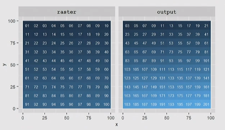
Local Operators

To perform simple mathematical operations

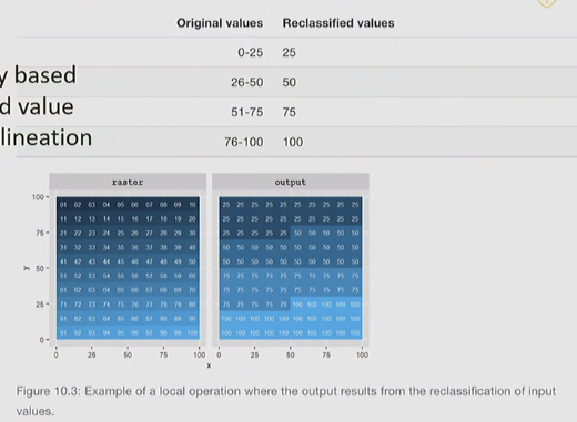
Example of local operation where output = (2 * raster +1)

Reclassification

To reclassify based on weighted value or other delineation

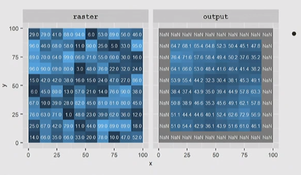
Example of a local operation where the output results from the reclassification of input values.

Focal Operation

-To smooth a surface; average based on neighbors; closer neighbors may be weighted

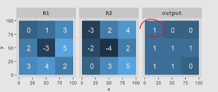
Example of a focal operation where the output cell values take on the average value of neighboring cells from the input raster. Focal cells surrounded by non-existent cells are assigned an NA in this example

Logical Comparison

To compare rasters to each other: Greater than >; less than <; equal to ==; not equal !=
Return a True (1, or any non-zero integer) / False(0) raster

Boolean (Logical)

To compare the true/false (conditional state) of raster after the logical comparisons
If whether statement you ask is TRUE, resultant raster cell will be 1;
Can be combined to find two rasters that meet requirements

Generalization of Raster Maps

Change resolution (increase or decrease cell size) for clarity
The smallest allowable size of groups of cell is the minimum mapping unit(MMU); combine cells below the MMU with neighbors to improve clarity.

Raster Overlay

Weighted Overlay

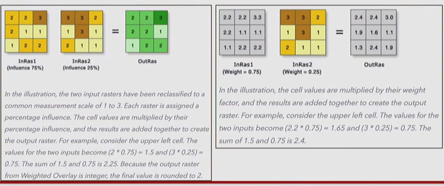
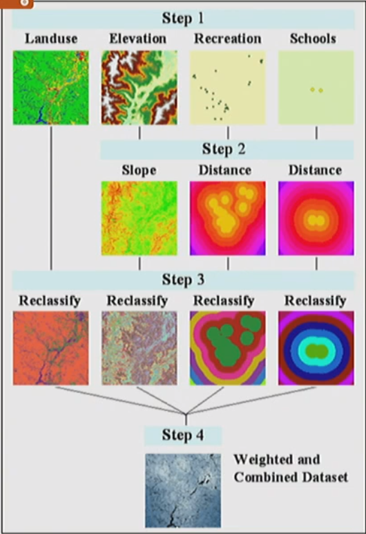
A method for aggregating layers of rasters by weighting the layers, multiplying each value by the weight, then adding. Two tools in ArcGIS Pro: Weighted Overlay(the output is always integer) and Weighted Sum (weight * value then add)

Site Suitability and Location

Site suitability analysis depends upon the ability to study characteristics of a location (and its nearby surroundings)

Reclassification

Before values from different rasters can be compared and analyzed together, they must be translated into a common measurement scale

Vectors and Rasters

Source data will likely consist of both vectors and rasters
For weighted overlay, analyses must be done to identify the correct information about the location and transform it into a raster

Networks, Path, and Accessibility

Networks problem

All types of network analysis/problems:
- Route planning and optimization: shortest or fastest route
- Finding a closest facility
- Identity the service area
- Vehicle-routing problems

Network vs. Lines

In a set of line features, such as a roads, the individual features are not aware of each other
When the lines are added to a network data set, rules of how the individual features are related to each other can be added
This called connectivity

Least-Cost Path Introduction

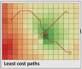
Least-cost path analysis is narrower than network analysis and is RASTER-based
In network analysis, movement through the network of vector features is measured and assessed based on rules of connectivity and measures of impedance
LCP has no defined path and a path is estimated based on values in raster cells

Creating the Cost Surface

Individual cost + individual cost = total cost value
Each type of cost is weighted against each other
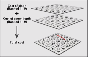
Your final cost raster can be the result of combining many types of data. The result is one final cost surface over which the cost of movement is measured.
With the accumulated costs and directions, the least cost path can be drawn from the source to destination sites.

Accessibility

Accessibility analysis of health care, emergency, or other social services studies the relative availability and distance of services to populations

Scale and Raster Analysis

Finding the Right Scale

Researcher need to choose what scale of data to work with for a given project
Scale of analysis should match the scale at which spatial processes operate- finer resolution data and larger scale is not always better.